Logistic Regression notes

In Linear Regression the goal is to find the equation of a straight line, plane or hyperplane which is the best fit or approximation to a set of data points (typically described by real values from a continuous range). From the derived equation it’s possible to interpolate or extrapolate to make predictions about data values not covered in the original data set (i.e. forecast the dependent / response variable (y) for any specified independent variable (x)). This works well where we have a linear relationship but how do we handle datasets where the response variable is not continuous but discrete (i.e. a small change in the independent variables (x) lead to a step, state or category change in ‘y’)?

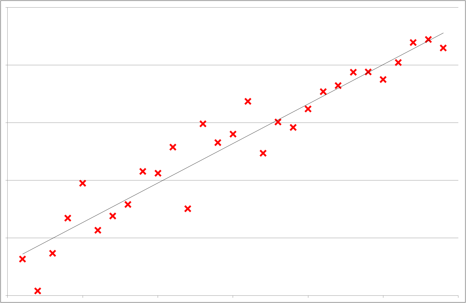
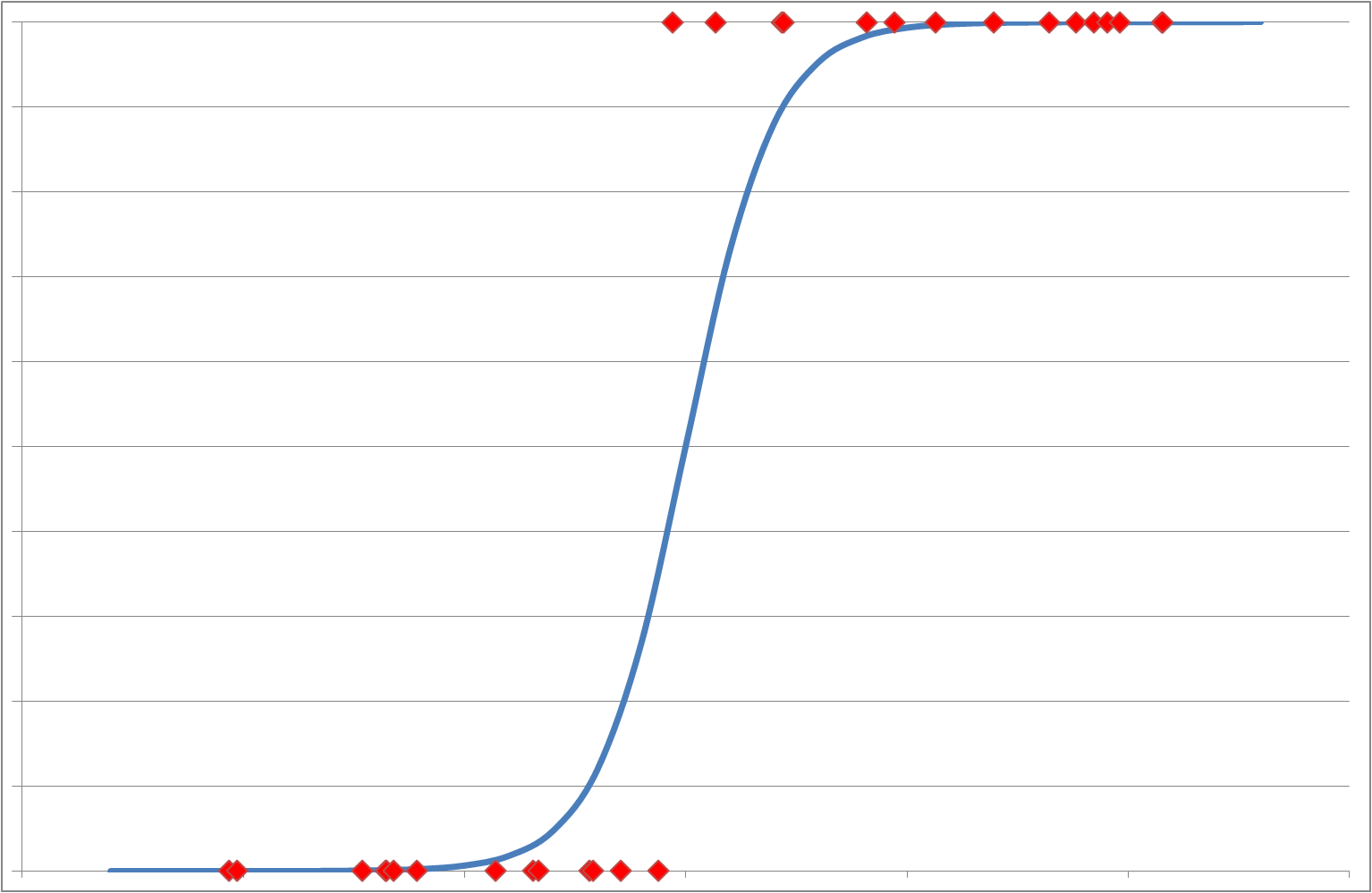
Figure 1: Comparison of linear and logistic regression graph profiles

The solution is ‘Logistic Regression’ which uses a mathematical function to cleverly convert input variables into one of two output states giving a BINARY (0 or 1) outcome. Depending on the context of the problem to which the approach is being applied these contrary states could be interpreted as a Boolean (True / False), On / Off, Success / Failure, Positive / Negative or some arbitrary categories A and B.

In the following example, I’m exploring ‘Binomial Logistic Regression’ – the term binomial referring to the model having 2 independent (input) variables. In this work I have labelled them x₁ and x₂. The principles can be extended to ‘Multinomial Logistic Regression’ involving multiple independent variables (x_i).

Mathematical Model discussion

In a one-dimensional linear model the equation takes the form:

$\mathrm{y}={\mathrm{\theta }}_1+{\mathrm{\theta }}_2\mathrm{x}$

For a two dimensional linear model, the equation of the plane would be:

$\mathrm{y}={\mathrm{\theta }}_1+{\mathrm{\theta }}_2{\mathrm{x}}_1+{\mathrm{\theta }}_3{\mathrm{x}}_2$

Higher order (multi-dimensional) linear models with multiple independent variables would give:

$\mathrm{y}={\mathrm{\theta }}_1+{\mathrm{\theta }}_2{\mathrm{x}}_1+{\mathrm{\theta }}_3{\mathrm{x}}_2+\mathrm{...}+{\mathrm{\theta }}_{\mathrm{n+1}}{\mathrm{x}}_{\mathrm{n}}$

where ‘θ’ is an array of constants and ‘n’ represents the number of independent variables (or dimensions). However, where trends or boundaries between regions are not linear more complicated polynomial equations are required to emulate curved shapes. Some example (non-linear) functions involving single independent variables are below:

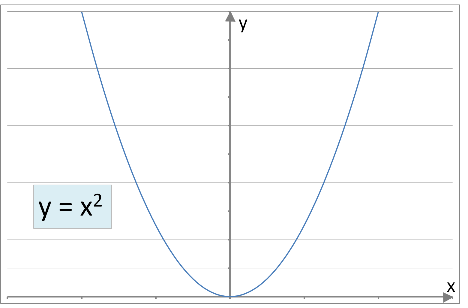
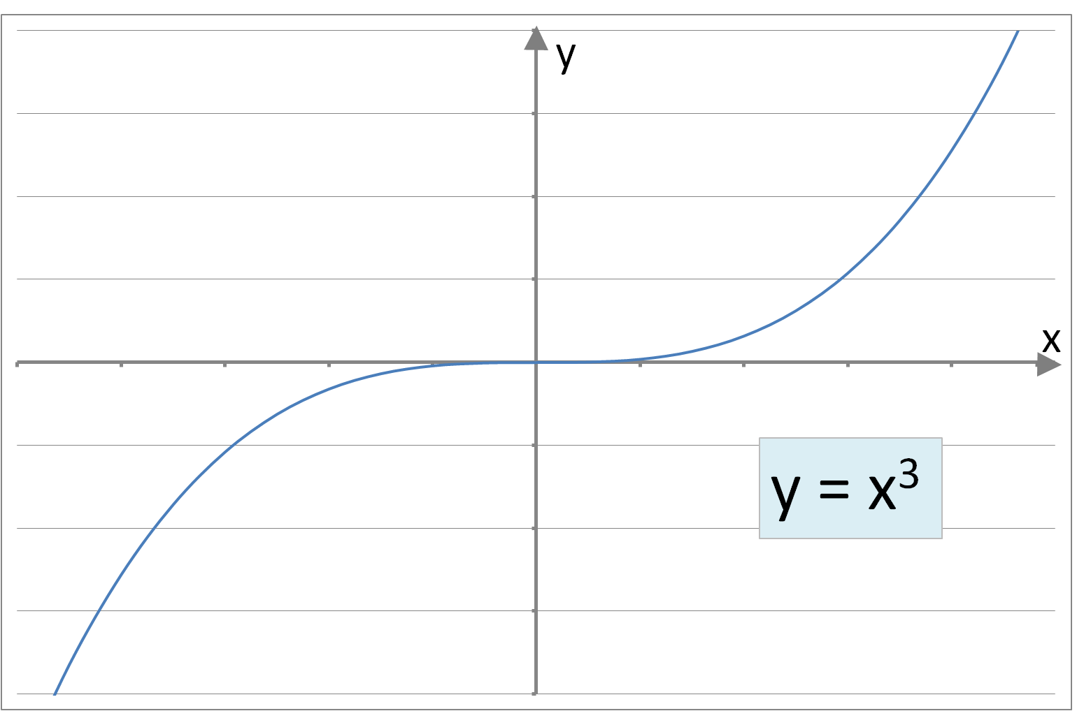
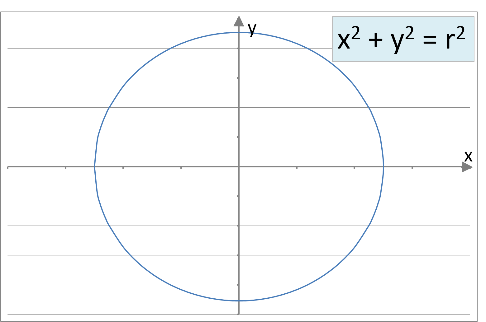
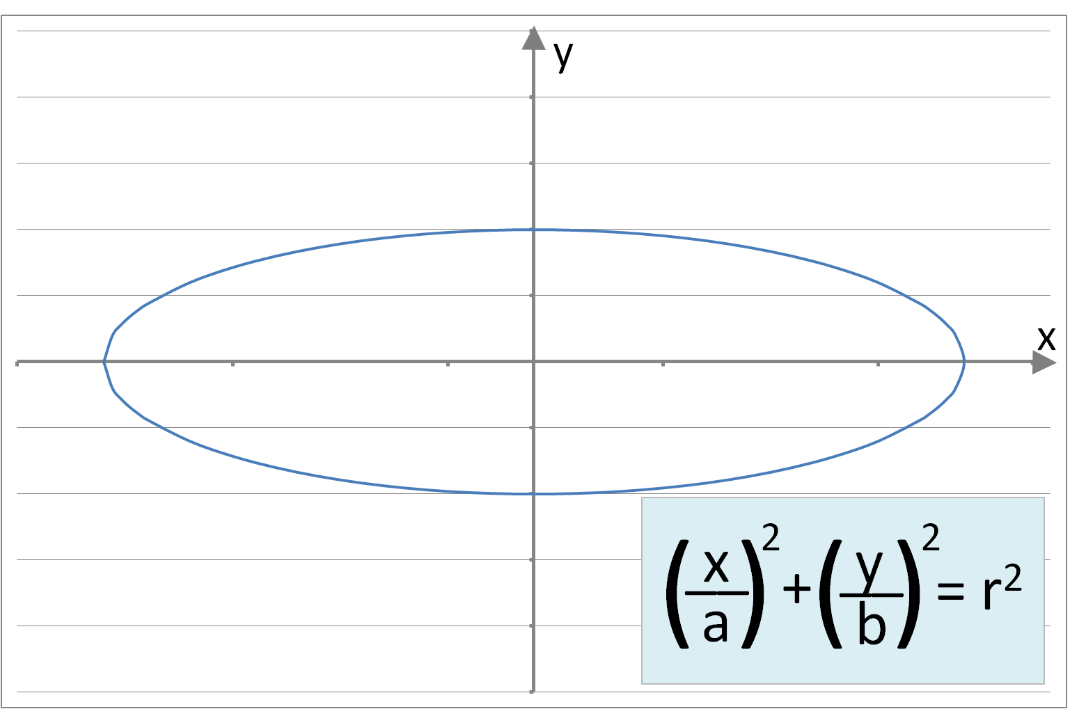
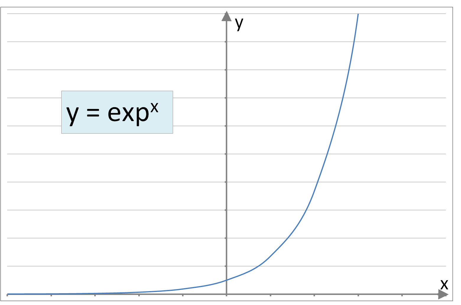
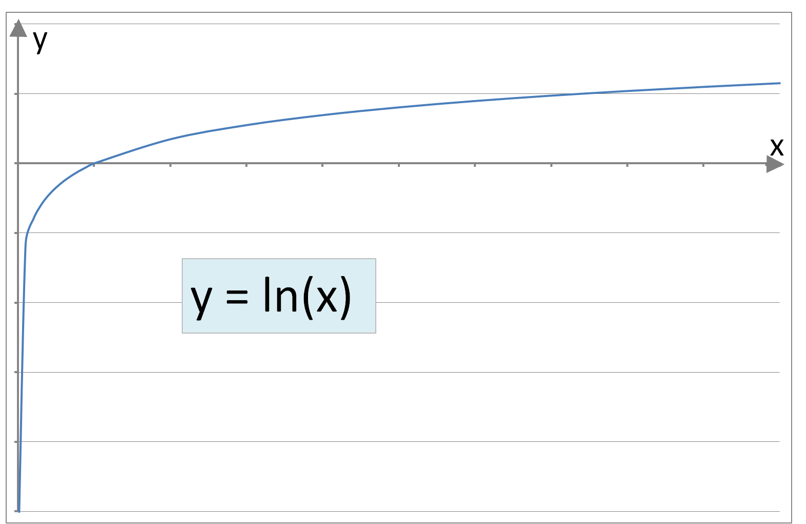
Figure 2: A sample of curve forms: Parabolic, Cubic, Circular, Elliptic, Exponential, Logarithmic, Square Root

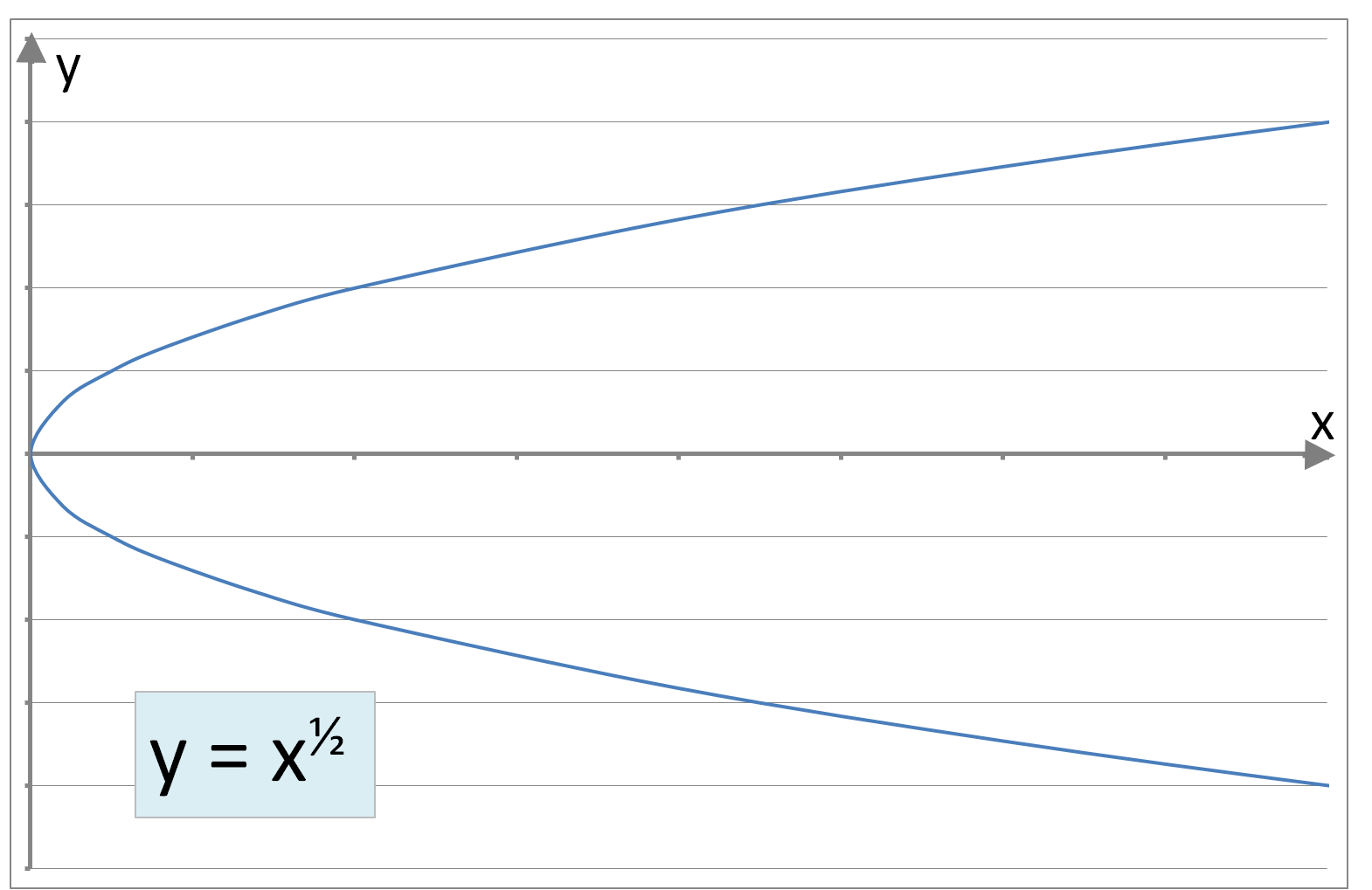
More elaborate curves can be generated by including different power terms in ‘x’ (e.g. x^½, x², x³) and, when there are two or more independent variables, mixed terms (e.g. x₁x₂). The generic form of such an equation with two independent variables would be:

$\mathrm{y}={\mathrm{\theta }}_1+{\mathrm{\theta }}_2{\mathrm{x}}_1+{\mathrm{\theta }}_3{\mathrm{x}}_2+{\mathrm{\theta }}_4{{\mathrm{x}}_1}^2+{\mathrm{\theta }}_5{\mathrm{x}}_1{\mathrm{x}}_2+{\mathrm{\theta }}_6{{\mathrm{x}}_2}^2+{\mathrm{\theta }}_7{{\mathrm{x}}_1}^3+{\mathrm{\theta }}_8{{\mathrm{x}}_1}^2{\mathrm{x}}_2+{\mathrm{\theta }}_9{\mathrm{x}}_1{{\mathrm{x}}_2}^2+\mathrm{...}+{\mathrm{\theta }}_{\mathrm{n+1}}{{\mathrm{x}}_2}^{\mathrm{n}}$

The values of θ_i are constants which can take positive, negative, large or small values providing a weighting to the variable terms (i.e. ${{\mathrm{x}}_1}^{\mathrm{j}}{{\mathrm{x}}_2}^{\mathrm{k}}$). Where a term has little influence on the dependent variable the value of the corresponding θ_i will be very small or zero.

For these models ‘y’ is continuous (i.e. ‘y’ can take any real number). However, in logistic models we are seeking an equation that yields discrete (or categorical) outcomes (e.g. at the simplest level a binary result of ‘y’ equals 0 or 1).

Logistic Regression is modelled mathematically using the Sigmoid function which forms an ‘S’ (or step) shaped curve (see Figure 2). Also known as the Cumulative Logistic Distribution it is expressed in the following way:

${\mathrm{H}}_{\mathrm{\theta }}\mathrm{(z)}=\frac{1}{\mathrm{(1+}{exp}^{\mathrm{-z}}\mathrm{)}}$

with a range of [0,1] and where ‘z’ is the independent variable. The symbolism H_θ(z) is used because the function describes a 'hypothesis' (model or representation) of the regression behaviour. This function has the distinctive property that for the majority of negative values of ‘z’ it gives a response of 0 and for positive ‘z’ values gives a response of 1 but for a narrow transition region (either side of z = 0) the result is ‘fuzzy’ and the calculated response could be assigned to 0 or 1 depending on the user defined criteria (or thresholds). For example:

	If Hθ(z) ≥ 0.5:	set Hθ(z) = 1
	If Hθ(z) < 0.5:	set Hθ(z) =0

Figure 3: Sigmoid Function (Cumulative Logistic Distribution)

Bringing these two mathematical concepts together, we can use a rich equation comprising multiple ‘x_i’ power terms and θ_i constants to calculate ‘z’:

$\mathrm{z}={\mathrm{\theta }}_1+{\mathrm{\theta }}_2{\mathrm{x}}_1+{\mathrm{\theta }}_3{\mathrm{x}}_2+{\mathrm{\theta }}_4{{\mathrm{x}}_1}^2+{\mathrm{\theta }}_5{\mathrm{x}}_1{\mathrm{x}}_2+{\mathrm{\theta }}_6{{\mathrm{x}}_2}^2+{\mathrm{\theta }}_7{{\mathrm{x}}_1}^3+{\mathrm{\theta }}_8{{\mathrm{x}}_1}^2{\mathrm{x}}_2+{\mathrm{\theta }}_9{\mathrm{x}}_1{{\mathrm{x}}_2}^2+\mathrm{...}+{\mathrm{\theta }}_{\mathrm{n+1}}{{\mathrm{x}}_2}^{\mathrm{n}}$

and then use the result in the Cumulative Logistic Distribution (Sigmoid) function to determine the binary response at each ‘x_i’ or combination of ‘x_i’s:

$\mathrm{y}~{\mathrm{H}}_{\mathrm{\theta }}\mathrm{(x)}=\mathrm{H(z)}=\frac{1}{\mathrm{(1+}{exp}^{\mathrm{-z}}\mathrm{)}}$

We will have a starting dataset that provides the x_i values and the associated ‘y’ responses. And our goal would be to obtain an equation that allows us to predict ‘y’ given some previously unseen ‘x’ values - with a level of accuracy that we can measure. In order to do this we need to derive appropriate values for the constants (θ_i) and to achieve this we can use a similar iterative, optimisation approach as we used for Linear Regression.

The Logistic Regression Cost function (which provides a measure of the deviation from the ideal solution and which we will seek to minimise) has a detailed derivation based on maximising the likelihood of outcomes. Also known as the log-likelihood equation, it is expressed in the following way:

$$\mathrm{J(\theta )}=-\frac{1}{\mathrm{m}}\sum _{i=1}^m\mathrm{(y\; log}{\mathrm{H}}_{\mathrm{\theta }}\mathrm{(x)}\mathrm{+\; (1-y)\; log\; (1\; –}{\mathrm{H}}_{\mathrm{\theta }}\mathrm{(x)))}+\frac{\mathrm{\lambda }}{\mathrm{2m}}\sum _{j=2}^{\mathrm{n+1}}{{\mathrm{\theta }}_j}^2$$

where ‘m’ is the number of data points and 'λ' is the Regularisation constant. The term $\frac{\mathrm{\lambda }}{\mathrm{2m}}\sum _{j=2}^{\mathrm{n+1}}{{\mathrm{\theta }}_j}^2$ is the Regularisation term. Its inclusion in the cost function is a means of controlling the size of the values determined for the 'θ' weightings. Effectively it adds a penalty to the cost function: if the θ weightings are large this term dominates and the cost increases; smaller values of θ incur a lower cost penalty which supports the goal of minimising the overall cost. Regularisation addresses the specific problem of ‘over-fitting’ where the polynomial equation defines a precise and accurate boundary (delineating categories within the known dataset) but consequently works less well as a general predictor for new data points.

Where the gradient (or steepness) of the Cost function is zero or close to zero the cost will be minimised (see Figure 6). The gradient is measured by the ‘change in y’ divided by the ‘change in x’ (denoted $\frac{\mathrm{dy}}{\mathrm{dx}}$) and can be determined mathematically using Differentiation. The Gradient function is given by:

For j=1:

For j=2 to n+1:

To be clear, 'i' is an index for each data point (1 to 'm') and 'j' an index for each 'θ' dimension (1 to 'n'+1). Finally, we need to update the values of theta (for j=1 to n+1):

$${\mathrm{\theta }}_j={\mathrm{\theta }}_j-\mathrm{\alpha }\frac{\mathrm{\partial }}{\mathrm{\partial }{\mathrm{\theta }}_j}\mathrm{J(\theta )}$$

Recall from our Linear Regression work that 'α' is the Learning Rate which can be adjusted to alter the rate of convergence.

Data Source

There are many existing data sources available which are commonly used to demonstrate the principle of Logistic Regression. Rather than simply reproducing analysis performed by other Data Scientists I decided to create a bespoke dataset. I developed a simple Excel programme that allowed me to specify the number of data points, the number of data point dimensions, the range of values (lowest to highest) in each dimension, and assign a category (e.g. ‘0’ or ‘1’ for a 2-state response) against each data point according to whether specific criteria are met.

For this randomly generated dataset, the category was set to ‘1’ where the data point was within a pre-defined region (an ellipse around a central point). As this would create a hard or clear boundary between categories I added a degree of variability in the assignment near the envelope edge. The 2-dimensional dataset and response variables used in this study can be downloaded. A visualisation of the data can be seen in Figure 4.

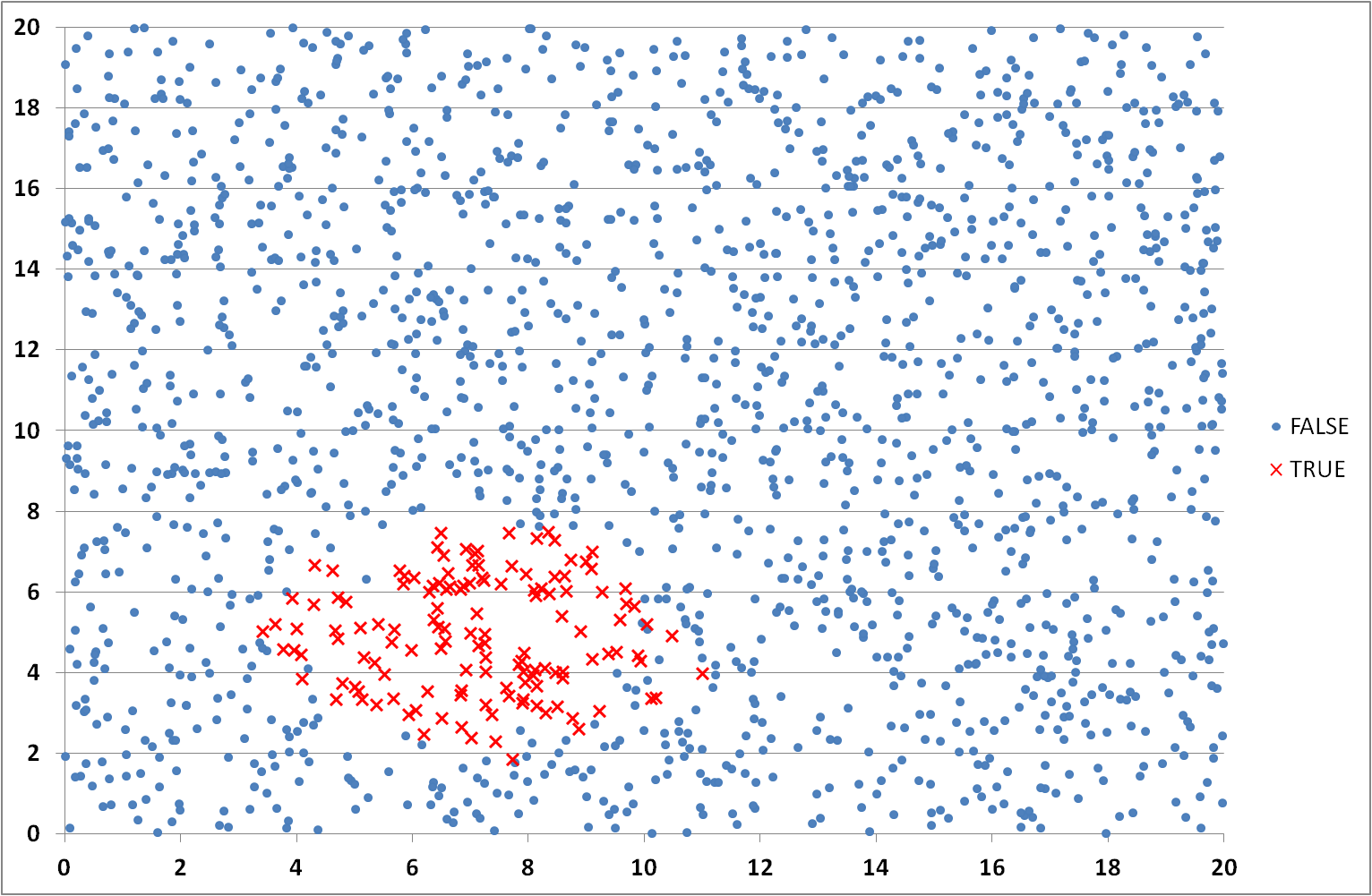
Figure 4: Dataset visualisation showing distribution of (True/False) categories

Process Flow

With the equations defined we need to assemble the sequence of activities required to create the computer programme. The workflow below outlines the blocks of functionality that the programme will need to perform.

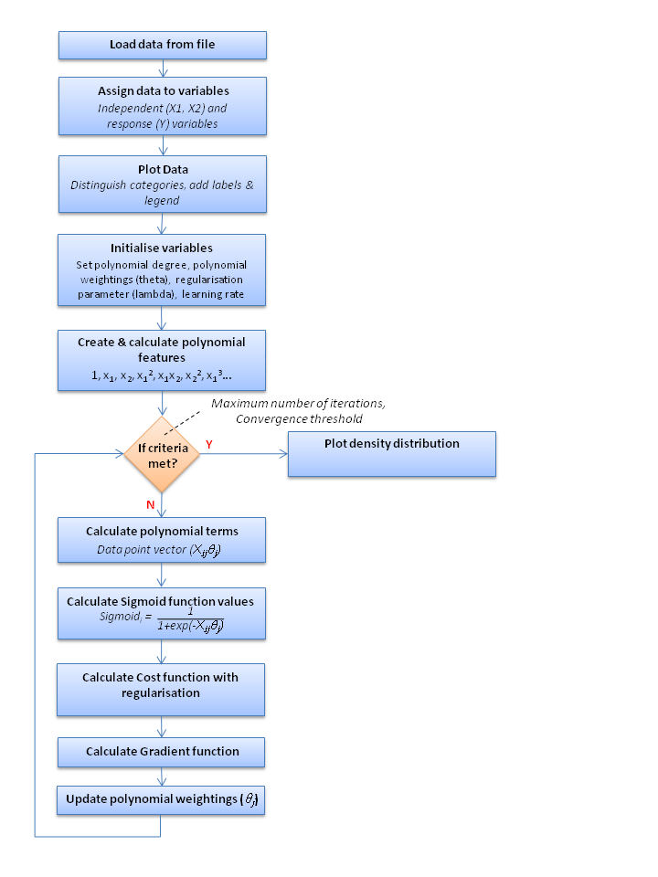
Figure 5: Logistic Regression programme workflow

Excel

There is no doubt that Excel is a great tool for analysing and visualising data but not naturally one that Data Scientist's turn to when seeking to solve complex vector multiplication problems or challenges requiring iterative or convergence capabilities. However, Excel's VBA toolkit provides an environment where linear (single-threaded) programmes can be developed. While VBA is not optimised for such vector computational work it does allow the Logistic Regression equations above to be programmed. Furthermore, in the absence of the in-built libraries of tailored platforms (like Python, R, SSPS, SAS, Stata, MatLab and Octave) it means that rather than relying on a 'black-box' to deliver a converged solution I have to understand the optimisation parameters and algorithms, and implement them successfully. This provides a valuable opportunity to fully explore the features and interactions of the polynomial equation, weightings, Cumulative Logistic Distribution, cost function, and gradient descent.

A copy of the Excel spreadsheet and VBA code can be downloaded from here. The tool has parameters that can be modified on the 'InputParameters' worksheet such as the highest order of polynomial terms (i.e. degree of features), the initial values of θ_i, the regularisation constant (λ), the learning rate (α), the Sigmoid threshold, the number of programme iterations to perform and whether to scale the 'x_i' values. The (x₁, x₂ and y) data values can be entered on the 'Dataset' worksheet. To use the tool macros need to be enabled.

The animation below illustrates the results achieved using the tool (with feature degree = 6, α = 1 and λ = 0.005) showing the declining cost and the developing prediction profile as the number of iterations increase. The model appears to converge and produce a stable solution after about 300K iterations (after the 'elbow' of the cost curve which occurs around 150K iterations).

Learning

I ran the programme for a total of 1 million iterations (which on a computer with an Intel i5 processor took 10 hours!). Clearly, taking a linear computing approach to such mathematical problems and algorithms is not efficient. As the array sizes for the number of data points, independent variables and polynomial complexity increases the number of calculations will increase unmanageably.

One problem I encountered early in my coding implementation was an error in calculating the Sigmoid function (H_θ(z)). With values of 'x' in my example dataset lying between 0 and 21 and with a polynomial of degree 6, values calculated for 'z' become very large (i.e. (21)⁶ which is of the order 10⁷). Calculating the exponential term within H_θ(z) (i.e. e^-z) gives such a large number that it could not be evaluated. However, it is reasonably intuitive to take the next step and recognise that if e^-z is very large, the value of H_θ(z) must be a good approximation to zero. So how can this problem be overcome?

The only way to ensure the polynomial does not generate excessively large numbers is to constrain the values of 'x' to the range -1 ≤ x ≤ +1. Consequently, the individual terms (${{\mathrm{x}}_1}^{\mathrm{j}}{{\mathrm{x}}_2}^{\mathrm{k}}$) will also be restricted to this range, regardless of the polynomial power, in order for H_θ(z) to be calculated. The standard technique adopted is to scale all the 'x' values in the dataset (i.e. if the largest absolute value of 'x₁' is 21, divide all values by 21). This linear scaling or mapping does not materially alter what is being calculated but you need to remember to interpret or re-scale the results produced by the programme.

The figure below demonstrates the impact of changing the learning rate within the model. Generally, an increase in the value of the learning rate (α) results in bigger changes to the polynomial constants (θ) and quicker convergence of the cost function. By tailoring this value the programme can run more efficiently. However, there is a threshold in the learning rate beyond which the algorithm becomes unstable and the cost diverges - in this case a value over 50. The most appropriate value to choose for each data set and logistic regression problem requires exploration.

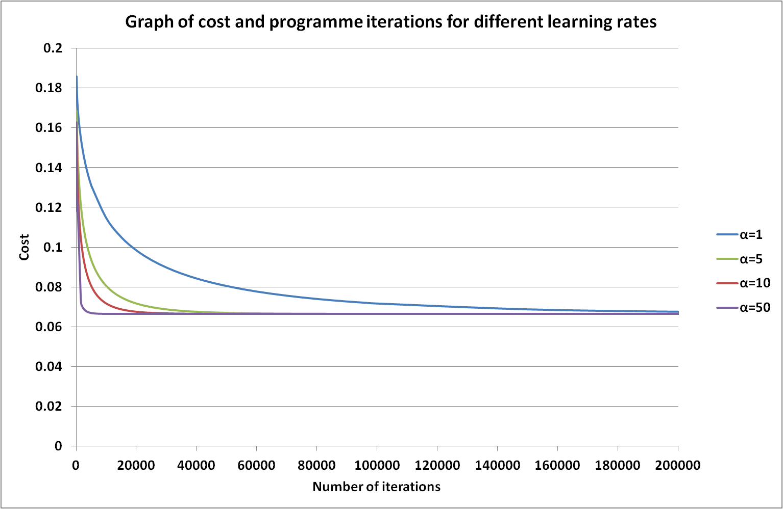
Figure 6: Rate of cost convergence as a function of the number of iterations and learning rate

Octave and Matlab

The same mathematical principles and algorithms outlined above can be applied in Octave (or Matlab). In the main procedure loop (see Figure 7) I have initially replicated the approach used in the Excel VBA programme which iterates through the polynomial, Sigmoid, Cost, Gradient and θ calculation steps many times until a satisfactory result is achieved. There are two options: (A) iterate a very large number of times (and hope the resulting values represent a stable solution and the cost minimised) or (B) repeat until the sum of the gradient terms (which is a measure of the deviation from the minimum cost) converges or reaches some specified value.

The former is somewhat arbitrary as too few calculations, while efficient, may not yield a convergent solution whereas too many calculations can be costly in time and processing power. In the latter, it may not be clear at the outset what convergence threshold to use: too large and the solution may not have stabilised or minimised and too small and the programme may never converge. Clearly, for both, an investigation of the impact of the number of iterations and convergence threshold parameters is needed.

The whole algorithm is described in the following procedures and functions (Figures 7 to 13).

Figure 7: Octave Code main procedure

Figure 8: Octave Code Cost Regularisation function

Figure 9: Octave Code feature mapping function

Figure 10: Octave Code decision boundary plotting function

Figure 11: Octave Code data point plotting function

Figure 12: Octave Code logistic regression prediction function

Figure 13: Octave Code Sigmoid function

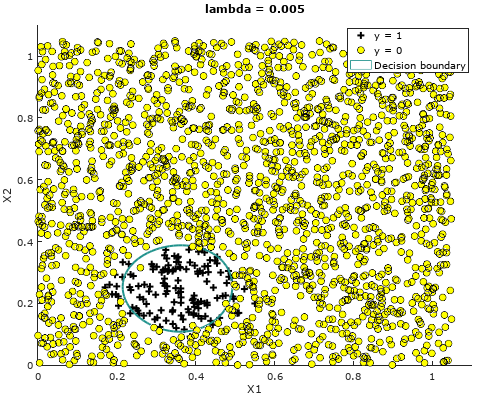
Figure 14: Logistic Regression Decision Boundary derived using Octave

The benefit of application toolsets like Octave, R and Python is that libraries of procedures have been developed and are readily accessible through simple procedure calls. Functions like FMINUNC in Octave are optimised to find the minimal cost without the need for the user to implement iterative routines. The main loop (see Figure 7) and Cost function with Regularisation (see Figure 8) could be replaced with the code using the FMINUNC function (see Figure 15).

Figure 15: Replacement Octave Code main procedure

Implementing the algorithm in VBA requires the use of one and two dimensional arrays to describe the polynomial, Sigmoid, cost, gradient and θ data. Because of the number of variables the developer must be disciplined in the implementation of the calculations to ensure the correct array elements are applied appropriately. This necessitates a careful understanding of the arrays and the equations they are used in. While this can give the developer a deep appreciation of the arrays and variables used in the algorithm at each iterative step it is time consuming to produce the code and is prone to implementation error.

Octave provides an improved solution in vector and matrix operations where calculations can be performed on matrix arrays or vectors in a simple way without having to address individual array elements. Consider the following comparison of coding examples. In traditional programming the multiplication of two arrays would require element-by-element calculations (in this case to determine the sum of the products of the 2D array 'Xmatrix' and 1D vector 'θ').

For i = 1 To numberOfDataPoints
 For j = 1 To numberOfPolynomialTerms
  thetaX(i) = thetaX(i) + (Xmatrix(i, j) * theta(j))
 Next j
Next i

But in vector programming tools this calculation is performed efficiently in the single command ThetaX = Xmatrix * Theta. An appreciation of matrix-vector multiplication is key to understanding how these arrays can be combined - a prerequisite to being able to multiply arrays is that the number of columns in Xmatrix (the left hand matrix) must match the number of rows in Theta (the right hand vector). In vector maths there is a need to understand the dimensions of the matrices and what they represent. For example, these are the sizes of the arrays used in the algorithm above:

• X (1..number of datapoints,1..2)
• y (1..number of datapoints)
• θ (1..number of polynomial terms)
• Sigmoid (1..number of datapoints)
• Grad (1..number of polynomial terms)

R

So how does R compare? One of the strengths of R is the comprehensive range of libraries with configurable parameters that can be called to perform tasks such as importing and plotting data, generating polynomials, and applying in-built Logistic Regression models to seek a solution. Consequently, once you have learnt the general principles of coding in R and RStudio it is relatively easy to locate and implement suitable procedures that perform the required functions.

R code is efficient - both in terms of the brevity of the code (see Figure 16) and the time taken to execute (a few seconds compared with minutes for the equivalent operations in Octave). This is primarily due to the highly developed nature of the R libraries.

Figure 16: Logistic Regression programme in R

The sequence of steps in R broadly follows the process in Figure 5 but the iterative steps to produce the polynomial terms and create and apply the Logistic Regression model are simpler, single commands - the complexity being handled within the R procedure calls. The following table describes the R commands used:

	Library	The procedures and functions available from R are grouped into related Library packages. In order to use specific collections of functionality users need to install the relevant code (using the command install.packages("library_name")) and then load the library (library("library_name")). In the above programme two libraries (readxl and ggplot2) are treated in this way.
	read_excel	This is a procedure that allows data to be imported from an Excel workbook. By default the import routine assumes the source data file includes a header row with labels / names for each column of data. As my dataset is unlabelled the col_names=FALSE parameter has to be set to avoid the first line of data being read and interpreted as field names. Other procedures are available for importing data from other file types (such as CSV, tab separated variables, web logs and tables).
	dim	This command takes an array as a parameter and displays the dimensions of the vector or matrix. While not necessary in the Logistic Regression programme it is always a useful check to perform to ensure the data expected has been imported.
	names	Where it is necessary to label the columns of a dataset or matrix the names function will apply the text strings provided as parameters. It assigns or re-names each column in the order given. Field names are required in order to inform R which columns of data should be used or operations applied to.
	data.frame	As in Python, data frames represent collections of data variables. R uses these structures as the basis of its operations and consequently loose sets of data need to be converted to this form (using the data.frame command) before some procedures can be used.
	ggplot	R offers a flexible plotting package for drawing multiple graph types, such as line graphs, scatter plots, histograms, box-plots, and offering functionality that allows data points, labelling, axes, legends and plot areas to be highly customisable. Here is a great introductory tutorial to ggplot.
	as.factor	The imported data set comprises three variables - two are real values (X1, X2) while the third is the (integer) response variable (Y) taking values of 0 (false) or 1 (true). In order to inform R that the latter variable represents a category rather than a continuous variable the as.factor command is applied to the data field holding the 'Y' values.
	geom_point	In order to generate a scatter plot the geom_point function is called to draw a point at each (X1,X2) coordinate of the dataset.
	scale_color_manual	This command allows R to set colours automatically for each data point based on the response value (Y). Colour is parameterised as a range (blue to red) so R can assign a colour for each category. In this dataset only two colour values are required.
	poly	Another powerful function is poly which takes a matrix comprising more than one column and creates polynomial (multiplicative) combinations of these columns (e.g. X1 * X2, X12). The function takes a parameter which defines the order (highest power) of the polynomial. This is equivalent to Octave's mapFeature function in Figure 9.
	as.matrix	This function converts a dataset or data frame into a matrix form. This is useful where the dataset is used as a parameter in a function expecting a matrix (such as poly).
	cbind	Where multiple datasets need to be combined into a single matrix the function cbind can be used. It can take many arguments, each representing a vector or matrix array that needs to be included in the combined dataset.
	sprintf	The sprintf function will be recognisable to anyone familiar with the C programming language as a tool for formatting text strings. In the above implementation there is a need to provide names or labels for each of the 27 columns of data generated in the poly function. By default the poly function does not provide column names and if labels are not added R has difficulty distinguishing the fields. sprintf is used as a succinct way of assigning names 'x01','x02',...'x27' to the columns in the array xfinal.
	glm	Another example of the power of R is the glm (Generalised Linear Model) procedure which takes as parameters the desired type of regression (Binomial Logistic Regression family), the data frame over which the algorithm is to applied (xfinal) and the response variable(s) (Y). The term (Y~.) has a special meaning that the Logistic Regression should be developed with the response (Y) a function of ALL other variables in the data frame.
	glm.control	As observed in the VBA and Octave examples, the regression algorithms are iterative, repeating calculations until the solution converges or a specified number of iterations have been performed. The glm.control function allows values to be specified for the convergence threshold and the maximum number of iterations.
	summary	The modelling function will generate statistics that are characteristic of the dataset and applied model. This is not an essential part of the Logistic Regression programme but for the user who can interpret the statistics can provide a valuable insight to the model fit (such as quartile distributions, the calculated coefficients, normal distribution density function (z), the number of iterated steps and a measure of the fit).
	predict	Having created a predictive model from the original dataset the predict procedure allows response values (Y) to be estimated for any specified (X1,X2) independent values. The procedure requires a model and set of data points over which to predict responses.
	expand.grid	As the objective is to apply the model to the range of values we started with (i.e. approximately X1 = 0 to 20 and X2 = 0 to 20) we require a function which can generate combinations of (X1,X2) coordinates that span this region. The expand.grid function accepts integer ranges for supplied variables (X1 and X2) and creates one row of data for each variable combination, effectively a grid of points. Note that as X1 and X2 values have been scaled to the range 0..1 and the expand.grid only deals with integers, the code uses X1 and X2 values between 0 and 100 and then scales them to get decimal increments of 0.01.
	contour	The contour function makes use of the predicted values (predictmodel) on the specified plot region (x=1..20,y=1..20) and generates a (grey) contour line wherever the response value is 0.5.
	points	The original dataset value pairs (X1,X2) are added to the contour plot using the points function which draws blue circles where the X1,X2 pairs have a response value (Y) of 0 and a red circle where the response value is 1.

And with R's help the result of all our hard work is...

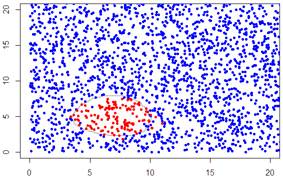
Figure 17: Plot of data points and decision boundary

Subjectively, the results illustrated in Figure 17 show reasonable agreement with the decision boundary derived using the other machine learning tools. However, it is vital to understand important differences in the Octave and R (in-built) models. The glm algorithm does not include regularisation but employs weighting terms to iteratively adjust the predicted mean until convergence is achieved.

A measure of the accuracy of each scheme can be achieved by splitting the data into Training, Evaluation and Test datasets. Each model can be built using the Training dataset and then the performance checked using the data set aside for Evaluation (i.e. calculate what percentage of the Evaluation data points are correctly predicted by the model). This is a useful step to assess whether the model parameters (such as the Regularisation constant) have been tuned to a specific (Training) data set rather than to operate well on the widest possible range of data. The model can finally be applied to the Test data in order to provide a percentage measure of predictive performance.

Practical Examples

There are a multitude of real world scenarios where the Logistic Regression technique is applied. Some interesting and eclectic case study examples which demonstrate the benefits and practical application of the method include:

• consumer and business credit risk assessments (Ref 1);
• analysing staff turnover (Ref 2);
• determining whether a customer financial transaction might be fraudulent (Ref 3, Ref 4);
• deciding whether a medical scan or biopsy test is indicative of a disease (Ref 5, Ref 6);
• Predicting educational attainment (Ref 7);
• Predicting customer purchasing behaviour (Ref 8, Ref 9);
• Social studies (Ref 10);
• Predicting landslide susceptibility (Ref 11).

Alternative Logistic Regression datasets

If you're interested in exploring Logistic Regression you may find the following publicly available datasets interesting to work with.

• Logistic Regression with UCI Adult Income (Kaggle)
• The Contraceptive Use Data / Wilner Housing Data / Copenhagen Housing Conditions (Germán Rodríguez, Princeton University)
• Bank Marketing Data (1010Data)
• Miscellaneous datasets (Department of Statistics, University of Florida)
• Machine Learning Repository (University of California, Irvine)
• Miscellaneous datasets for Stata, SAS, SPSS, Mplus and R (UCLA Institute for Digital Research and Education)
• KidCreative (LogisticRegressionAnalysis.com)

My understanding of the features of Logistic Regression were gleaned on Andrew Ng's Machine Learning course. To explore the principles of Logistic Regression further I would recommend this course.