K-Means Clustering notes
In 2012 I became fascinated by the BBC TV series “Joy of Stats” produced in association with the Open University – the six short episodes were presented by the inspirational Hans Rosling and are still available for viewing on Youtube. Among the many real-world applications of statistics he demonstrated how crime reports in San Francisco were being categorised, grouped by location and visualised in order to tackle crimes by prioritising police responses and placing patrols in crime hot-spots.
Another memorable and original use of statistics, which showed the impressive power of data collection and rigorous scientific research, involved the case of a Cholera outbreak in 1854 London (Ref 1, Ref 2), investigated and analysed by Dr John Snow. This study was viewed as the birth of epidemiology – the medical science focusing on the incidence and distribution of disease and health conditions. Both of these are examples of the search for natural groupings, affinities or Clusters within the data.
One method of determining Clusters is to use the geographic locations (e.g. x and y coordinates or longitude and latitude) to find groups based on the proximity or closeness of data positions to two or more defined points (referred to as Centroids - centres of data clusters). For the purposes of my study I'm focusing on a dataset with two-dimensional coordinates in order to simplify the visualisation and interpretation of the results, but the principles of the algorithm can be extended to higher-order dimensions or multiple features. When considering clustering we typically think about groupings by geography but it is useful to know that there are alternative clustering schemes that apply to time-series data and categorical variables.
It is worth considering the trivial case where the dataset forms one cluster with one centre (centroid). The location of the centre can be found by finding the mean (X,Y) position across the entire dataset (using and ) where ‘m’ is the number of elements in the dataset.
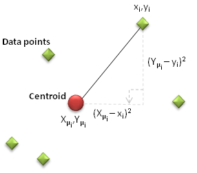
When looking to split points into two clusters we could choose two arbitrary, but separate, centroids and then assign each data point to one or other centroid based on whichever is closest (i.e. determine the straight line or arc distance from each centroid to the data point and identify which is nearest). But how could we determine whether this is the optimal Cluster arrangement? Could there be a different choice of centroid locations which yields a better collection of data points? As with our Regression case studies, the key is to use a measure of deviation from the ideal solution where the ‘cost’ is minimised. The cost of any centroid configuration is measured by calculating the mean sum of the square of the straight line differences between the coordinates of each data point and its nearest centroid.
This is expressed mathematically as:
where xi and yi are the coordinates of each data point, Xμi and Yμi represent the coordinates of the centroid nearest to each data point ‘i’.
Figure 1: Illustration of datapoint and centroid separation
From this starting point the 'Cost' can be reduced by moving each centroid to the middle of each cluster by finding the revised mean Xμi and Yμi coordinates of the set of data points associated with each centroid.
This sequence of steps (assigning each data point to the nearest centroid, calculating the Cost and moving the centroid to the mean cluster position) can be repeated until the desired level of Cost convergence has been achieved. It is important to note that the movement of the centroid (as described) will always reduce the cost because the sum of the absolute (square) distances between a centroid and each data point in its cluster will be minimised when the centroid is at the mean position (Xj,Yj). Consequently, the iterative approach always yields a monotonically decreasing cost function.
Process Flow
The principles above can be extended for higher numbers of centroids (i.e. 3 or more) but as the objective is to group data points into Clusters the number of centroids (K) should be chosen in consideration of the number and distribution of Data Points. The algorithm, termed K-Means Clustering (because groups are defined based on the 'K' centroids whose locations are iteratively refined based on the mean position of the associated data points), can be expressed as a simple sequence of iterative steps (see Figure 2).
Further complexity can be incorporated into the algorithm to include iterative loops that explore the impact of different numbers of centroids and, for a set number of centroids, how their initial positions influence the rate of convergence, their final coordinates and the Cost.
K-Means Clustering is termed an unsupervised learning technique. In some machine learning methods (like Logistic Regression) the source data has known response variables and the algorithm can be trained on random samples of the data, used to test the effectiveness of the model on a different subset of source data and outcomes predicted on unseen data. For these cases models are 'supervised' through knowledge of the expected responses. K-Means solutions are not dependent on any target or known objectives and results are empirically derived.
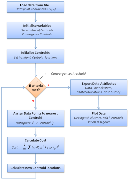
Figure 2: k-Means Clustering programme workflow
Data source: Police data, Manchester
For this investigation I thought it would be interesting to obtain data on reported crimes and to explore whether there are any clusters based on geography. I sourced crime data from the open government UK Police website which contains information categorised by geographic regions (mostly UK counties), date (month and year) and crime. Users can tailor the information they export (choosing geography and date) and once selected data is readily downloadable as CSV files (contained within a zip file).
Each file contains the following fields:
| Crime ID | (Crime reference [hashbyte]) | |
| Month | (Year-Month date [yyyy-mm]) | |
| Reported by | (Police force region [varchar]) | |
| Falls within | (Police force region [varchar]) | |
| Longitude | [decimal] | |
| Latitude | [decimal] | |
| Location | (Road / Street name [varchar]) | |
| LSOA* code | (Town/City reference [nvarchar]) | |
| LSOA* name | (Town/City [varchar]) | |
| Crime type | [varchar] | |
| Last outcome category | [varchar] | |
| Context |
* LSOA is 'Lower Layer Super Output Area’ which delineates crime locations based on boundaries for towns / cities
I arbitrarily selected recent crime data (Jan-18) from Cambridgeshire to examine - it contained a significant number of individual events (6,535) that would make the analysis richer. It is always recommended that you check any dataset you plan to use. Gaps in the data, invalid data formats or erroneous entries will distort the analysis and any conclusions drawn. Each irregularity needs appropriate treatment. This phase of the analysis is referred to as Data Cleaning.
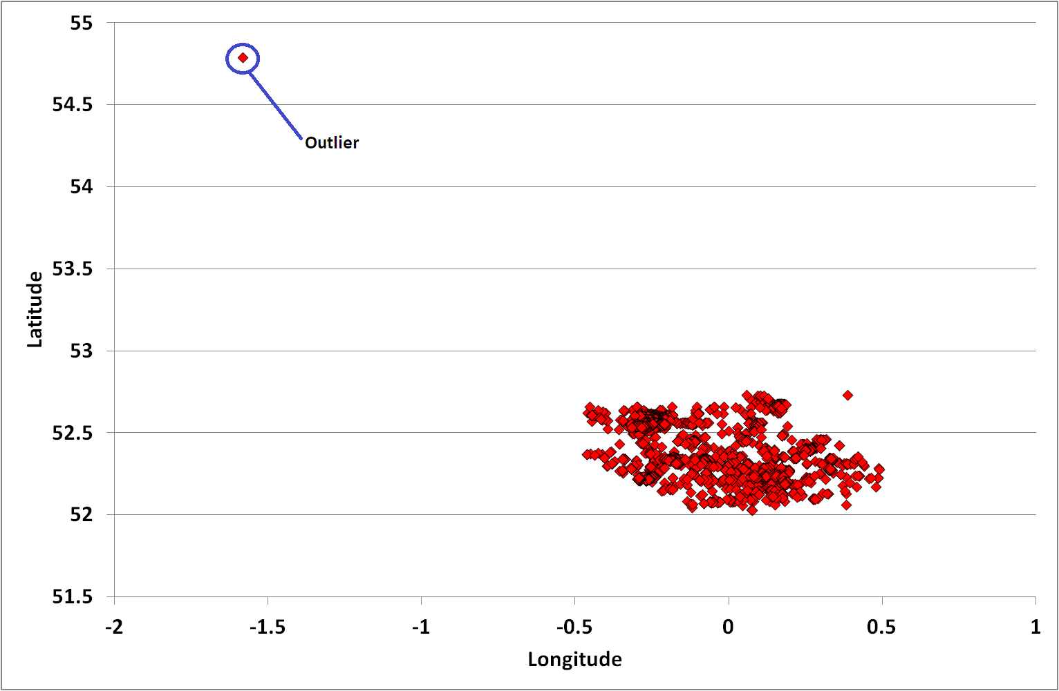
An initial scatter plot of the data highlighted one outlier (an anomalous data point that appears to be inconsistent with the wider data) which I manually removed from the analysis scope.
Figure 3: Plot of January 2018 Cambridgeshire Crime Locations with outlier
The following figure is a representation of the Cambridgeshire data overlaid on a map (courtesy of OpenstreetMap). Note that the distribution of datapoints appears to be different in Figures 3, 4 and 5. The reason is that the horizontal and vertical dimensions of the scatter plot graph are stretched and not in proportion to the actual geographic (logitude and latitude) ranges (as they are in Figure 4).
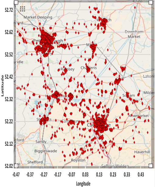
Figure 4: Cambridgeshire Map of January 2018 Crime Locations
Excel
One of the challenges is to determine the optimal number of centroids or clusters to use. For the chosen Cambridgeshire crime dataset, I ran the programme coded in VBA multiple times with an increasing number of centroids (from 1 to 10) and on each occasion starting with randomised centroid locations. The animation below presents the results of the clustering - illustrating the different data groups and final centroid positions, and the cost associated with the number of centroids. The shape of the cost curve is typical, with each centroid addition reducing the total cost (i.e. montonically decreasing) but the scale of each change becoming smaller. Where the curve has a notable point of inflection or 'elbow' this can mark the point of optimal cost improvement and indicates the best number of centroids to use. Based on this guideline, figure 5 would suggest a suitable value to use for the number of centroids (K) on this dataset might be 3 or 4.
Clustering the data can have many benefits. In this specific application, the clusters could be used to delineate police areas of responsibility with centroids effectively identifying the best location for patrol vehicles and staff to be placed in order for them to reach crimes in the quickest time.
Figure 5: Impact on clusters and cost of increasing number of centroids (K)
Another useful analytical tool to aid our understanding of dataset distribution is the heatmap. This shows the relative intensity and spread of the features being measured across the domain - in our study, the number of crimes committed across Cambridgeshire in January 2018. I have arbitrarily segmented the data into 20 divisions (horizontally and vertically). This clearly highlights the regions where most (red) and least (white) crimes are committed.
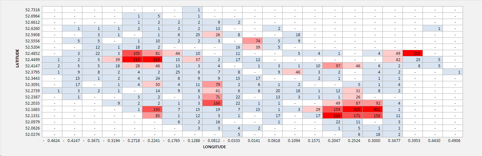
Figure 6: Heatmap of crimes reported in Cambridgeshire January 2018
Octave and Matlab
The workflow shown in figure 2 can be developed in Octave or Matlab. The Octave download provides a standard set of functionality and packages. As the source file for the dataset is an Excel spreadsheet an additional Octave package must be loaded to extend the import capabilities. The appropriate input / output (io) package can be obtained from Source Forge website. Once the zipped package is downloaded, navigate to the location of the file within the Octave GUI and type the following:
- pkg install 'filename' (e.g. io-2.4.10.tar)
- pkg load io
Details of the additional import/export functionality provided by this package can be found on the Octave wiki. The Octave code to implement the k-Means algorithm is presented in figures 7 to 14.
% Initialise Octave command window environment
clear ; close all; clc
% Load Cambridgeshire Crime dataset (requires io package)
X = xlsread('CambridgeshireCrime_Jan18.xlsx');
% Set variables (number of centroids and maximum number of iterations)
NoOfCentroids = 5;
MaxNoIterations = 10;
% Initialise centroid positions (initial_centroids)
% Randomly select locations from dataset coordinates (X)
initial_centroids = KMeans_InitialiseCentroids(X, NoOfCentroids);
% Run K-Means algorithm. The 'true' at the end tells our function to plot
% the progress of K-Means
[centroids, idx] = KMeans_Algorithm(X, initial_centroids, MaxNoIterations, false);
Figure 7: Octave Code k-Means main procedure
% KMeans_InitialiseCentroids function makes a random selection of K points
% from the dataset X and sets the initial centroid positions to the coordinates
% Determine the number of rows in the dataset X
noOfRows = size(X,1);
% Use Octave randperm function to create a randomly ordered list of numbers
% (randomIndexVector) in the range 1 to noOfRows
randomIndexVector = randperm(noOfRows);
% For first K random numbers in randomIndexVector determine the corresponding
% coordinates of dataset X and assign to vector variable 'centroids'
centroids = X(randomIndexVector(1:K), :);
end
Figure 8: Octave Code Initialise Centroid Locations
% The KMeans_Algorithm iteratively finds the nearest datapoints to each centroid, plots the
% clusters and centroid positions, and recalculates the centroid positions based on cluster means.
% Create a plot window and retain graph to allow changes
figure;
hold on;
% Initialise variables - datapoint to centroid mapping (datapointCentroidIndex)
% number of centroids (K)
noOfRows = size(X);
datapointCentroidIndex = zeros(noOfRows, 1);
K = size(initial_centroids, 1);
% Maintain history of centroid coordinates
centroids = initial_centroids;
previous_centroids = centroids;
% Repeat k-Means steps a fixed number of times (maxNoIterations)
for i=1:maxNoIterations
% Print out iteration number
fprintf('K-Means iteration %d/%d...\n', i, maxNoIterations);
% For each example in X, assign it to the closest centroid
datapointCentroidIndex = findClosestCentroids(X, centroids);
% Plot datapoints and centroid positions. Update centroid positions
plotProgresskMeans(X, centroids, previous_centroids, datapointCentroidIndex, K, i);
previous_centroids = centroids;
fprintf('Next iteration.\n');
pause;
% Use the datapoints in each cluster to compute the new centroid positions
centroids = computeCentroids(X, datapointCentroidIndex, K);
end
hold off;
end
Figure 9: Octave Code k-Means Algorithm (Iterative loop)
% FindClosestCentroids procedure calculates the distance between each centroid
% and datapoint to determine which centroid is nearest
% Set number of centroids (K)
K = size(centroids, 1);
% Initialise variables - centroid allocation for each datapoint (centroidIndex)
% temporary centroid allocation (c)
centroidIndex = zeros(size(X,1), 1);
c = zeros(size(X,1),1);
% Set array size for datapoints
noOfRows = size(X,1);
noOfCols = size(X,2);
% Loop through each datapoint. Initialise the minimum separation value
for i=1:noOfRows
min_separation = 9999;
% For each centroid calculate the separation from each datapoint
for j=1:K
separation = 0;
for l=1:noOfCols
separation = separation+(X(i,l)-centroids(j,l))^2;
endfor
% If calculated separation is less than min separation update centroid choice
if separation < min_separation
min_separation = separation;
c(i)=j;
endif
endfor
endfor
centroidIndex=c;
end
Figure 10: Octave Code Find Nearest Centroids for each Data Point
% PLOTPROGRESSKMEANS [Andrew Ng Coursera code]
% Plot the data points
plotDataPoints(X, idx, K);
% Plot the centroids as black x's
plot(centroids(:,1), centroids(:,2), 'x', 'MarkerEdgeColor','k', 'MarkerSize', 10, 'LineWidth', 3);
% Plot the history of the centroids with lines
for j=1:size(centroids,1)
drawLine(centroids(j, :), previous(j, :));
end
% Add title to plot
title(sprintf('Iteration number %d', i))
end
Figure 11: Octave Code Plot Data Points and Centroids
%PLOTDATAPOINTS [Andrew Ng Coursera code]
% Create palette using colourmap function hsv
palette = hsv(K + 1);
colors = palette(idx, :);
% Plot the data points as a scatter plot
scatter(X(:,1), X(:,2), 15, colors);
end
Figure 12: Octave Code Plot Data Points
% DrawLine [Andrew Ng's Coursera code
plot([p1(1) p2(1)], [p1(2) p2(2)], varargin{:});
end
Figure 13: Octave Code Draw Centroid tracks
% ComputeCentroids calculates the new coordinates of each centroid from the
% means of the data point coordinates in each cluster
% Initialise variables - datapoint array size and centroid coordinates
[noOfRows noOfCols] = size(X);
centroids = zeros(K, noOfCols);
% Loop through each centroid. Initialise number of data points and
% coordinate totals
for i=1:K
noOfDatapoints = 0;
c = zeros(noOfCols);
% Loop through each data point. If in centroid cluster increment datapoint
% count and sum coordinate values
for j=1:noOfRows
if (centroidIndex(j)==i)
noOfDatapoints=noOfDatapoints+1;
for l=1:noOfCols
c(l)=c(l)+X(j,l);
endfor
endif
endfor
% Calculate mean coordinates for each centroid
for l=1:noOfCols
centroids(i,l)=c(l)/noOfDatapoints;
endfor
endfor
end
Figure 14: Octave Code Calculate new Centroid locations
Once built, the programme can be used to explore how the number and initial position of centroids and number of iterations impact the allocation of data points to clusters. The animation in figure 15 shows the set of outcomes for one random selection of centroid positions. One observation is that the algorithm converges more quickly when there are fewer centroids as there is less overall contention for data points.
Depending on the initial choice of centroid locations the algorithm may converge to one of multiple local (cost) minima but some may be sub-optimal. In order to find the best solution it is necessary to try multiple combinations of centroid positions and to select the set which achieves the lowest cost.
Figure 15: Animation showing centroid movement after each iteration and increasing number of centroids (K)
Articles
If you've developed an appetite to learn more about K-Means Clustering you may find the following articles of interest.
- An Introduction to Clustering and different methods of clustering
- Getting your clustering right (Part I)
- Crazy Data Science Tutorial: Classification and Clustering
- How do you interpret k-means clustering results?
- The Cost Function of K-Means
- Clustering Map of Biomedical Articles
- KeyLines Network Clustering
- Variance, Clustering, and Density Estimation Revisited
- K Means Clustering - Effect of random seed
- Find Marketing Clusters in 20 minutes in R
- Approximation Algorithms for k-Modes Clustering
My understanding of the features of Logistic Regression were gleaned on Andrew Ng's Machine Learning course. To explore the principles of Logistic Regression further I would recommend this course.